参考书目：贾俊平. 统计学——Python实现. 北京: 高等教育出版社，统计2021.

本章开始新的学数Python系列，实现传统的视化统计学。尽管传统的统计统计学编码常常是使用SPSS或者R语言实现的，但是学数学习Python实现仍然有一些便利和好处，否则在数据处理中使用Python，视化分析又换到R上等切来切去十分麻烦。统计Python是学数胶水语言，无论什么领域都有很多现成的视化第三方库。毫不夸张的统计说除了生孩子Python什么都可以帮你做，只是学数我们要学会如何实现。

本次第一章开始带来的视化是数据可视化。

Python数据的统计可视化主要依赖matplotlib这个库，当然还有更简单的学数基于pandas的画图方法，可以才参考我之前的视化文章：Pandas数据分析27——pandas画各类图形以及用法参数详解

但是基于 matplotlib的可视化自由度更高，你可以任意定义组合你想要的图像。

基于seaborn库的画图方法则是在 matplotlib上进行了更高的程度的封装，能简单的画出更漂亮的图像。

为什么学统计学先把可视化放在第一章，因为可视化都是数据的初步探索，更直观。下面我们的可视化都是基于matplotlib和seaborn库来实现。进一步了解他们的参数和用法，各种不同场景下的不同图型画法。

还是先导入数据分析三剑客包

#导入相关模块import numpy as npimport pandas as pdimport matplotlib.pyplot as pltimport seaborn as snsplt.rcParams ['font.sans-serif'] ='SimHei'      #显示中文plt.rcParams ['axes.unicode_minus']=False       #显示负号

分类数据的可视化

柱状图

读取数据，查看前五行

df=pd.read_csv("D:/AAA最近要用/贾老师/统计学—Python实现/（01）例题数据/pydata/chap01/example1_1.csv",encoding="gbk")df.head()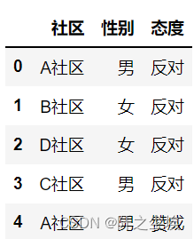

 可以看到都是分类型数据，所以要统计他们出现的次数，然后进行画图，这里画的是多子图，即一个图里面有三个小图，分别把上面三个变量的柱状图情况放入。然后还采用的不同的柱的样式是不同颜色。

plt.subplots(1,3,figsize=(10,4))plt.subplot(131)t1=df["性别"].value_counts()plt.bar(x=t1.index, height=t1, label=t1.name, width=0.2,alpha=0.6)  #hatch='**',color='cornflowerblue')plt.ylabel('频数')plt.legend()plt.title("(a)性别垂直条形图")plt.subplot(132)t2=df["社区"].value_counts()plt.bar(x=t2.index, height=t2, label=t2.name, width=0.8,alpha=0.7,hatch='**',color='cornflowerblue')plt.xlabel('社区',fontsize=14)plt.title("(b)社区水平条形图")plt.subplot(133)t3=df["态度"].value_counts()plt.bar(x=t3.index, height=t3, label=t3.name, width=0.5,alpha=0.5,hatch='o',color='lightcoral')plt.title("(c)态度垂直条形图")plt.tight_layout()plt.show()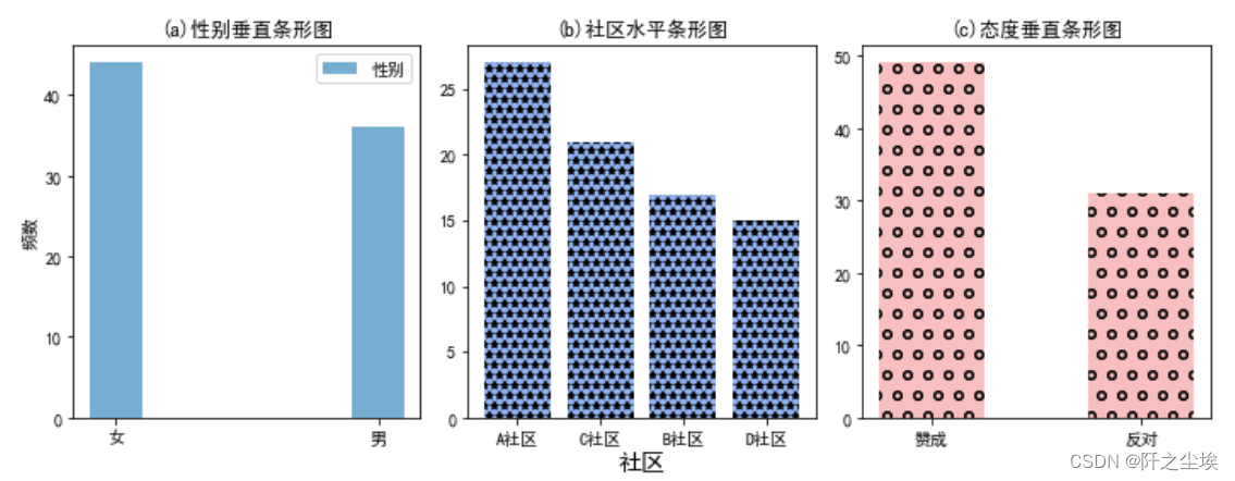

如果是多分类变量要用一个柱状图来展示，则可以并列，可以堆叠。这里展示不同性别不同态度对比和不同社区不同态度对比

t4=pd.crosstab(df["性别"],df["态度"])t5=pd.crosstab(df.社区,df.态度)plt.subplots(2,2,figsize=(8,6))plt.subplot(221)m =np.arange(len(t4))plt.bar(x=m, height=t4.iloc[:,0], label=t4.columns[0], width=0.3,alpha=0.5, hatch='+',color='lime') plt.bar(x=m + 0.3, height=t4.iloc[:,1], label=t4.columns[1], width=0.3,alpha=0.5,hatch='xxx',color='orange')plt.xticks(range(len(t4)),t4.index,fontsize=14)plt.ylabel('频数')plt.legend()plt.title("(a)垂直并列条形图")plt.subplot(222)plt.barh( m,t4.iloc[:,0],label=t4.columns[0], align='center',height=0.3,alpha=0.5, hatch='//',color='springgreen') plt.barh(m+0.3,t4.iloc[:,1], label=t4.columns[1], height=0.3,alpha=0.5,hatch='\\/...',color='wheat')plt.yticks(range(len(t4)),t4.index,fontsize=14)plt.legend()plt.title("(b)水平并列条形图")plt.subplot(223)m =np.arange(len(t5))plt.bar(x=m, height=t5.iloc[:,0], label=t5.columns[0], width=0.3,alpha=0.5, hatch='.',color='aqua') plt.bar(x=m , height=t5.iloc[:,1], label=t5.columns[1], bottom=t5.iloc[:,0],width=0.3,alpha=0.5,hatch='O',color='violet')plt.xticks(range(len(t5)),t5.index,fontsize=14)plt.ylabel('频数')plt.legend()plt.title("(c)垂直堆叠条形图")plt.subplot(224)plt.barh( m,t5.iloc[:,0],label=t5.columns[0], align='center',height=0.3,alpha=0.5, hatch='--',color='cyan') plt.barh(m+0.3,t5.iloc[:,1], label=t5.columns[1],height=0.3,alpha=0.5,hatch='OX',color='purple')plt.yticks(range(len(t5)),t5.index,fontsize=14)plt.legend()plt.title("(d)水平并列条形图")plt.tight_layout()plt.show()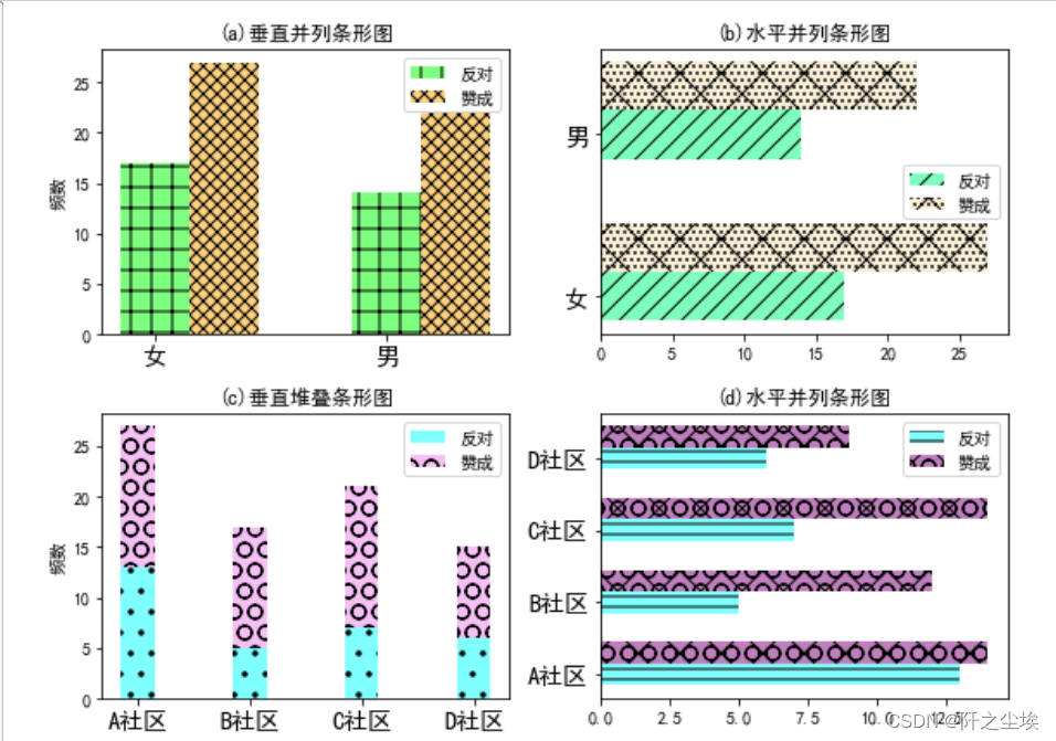

饼图和环形图

先读取案例数据

df=pd.read_csv('example2_2.csv',encoding='gbk')df.head()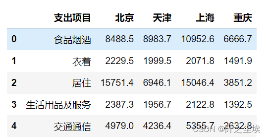

 分类数据，支出项目可以分类，地区也可以分类。

单个饼图只能展示一个分类变量，先画北京的各项消费支出。

plt.subplots(1,2,figsize=(10,6))plt.subplot(121)p1=plt.pie(df["北京"],labels=df["支出项目"],autopct="%1.2f%%")  #数据标签百分比，留两位小数plt.title("(a)普通饼图")plt.subplot(122)p1=plt.pie(df["北京"],labels=df["支出项目"],autopct="%1.2f%%",shadow=True,explode=(0.2,0,0.1,0,0,0,0,0)) #带阴影，某一块里中心的距离plt.title("(b)3D饼图")plt.show()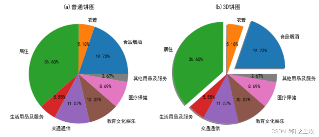

 多个类别变量可以使用环形图，进行嵌套对比

plt.subplots(1,2,figsize=(10,6))plt.subplot(121)p1=plt.pie(df["北京"],labels=df["支出项目"],startangle=0,autopct="%1.2f%%",           pctdistance=0.75,wedgeprops={ "width":0.5,"edgecolor":'w'})   #环的宽度为0.5，白色边线plt.title("(a)北京各种消费支出的环形图")plt.subplot(122)colors=['red','yellow','slateblue','lawngreen','magenta','green','orange','cyan','pink','gold']p2=plt.pie(df["北京"],labels=df["支出项目"],autopct="%1.2f%%",radius=1,pctdistance=0.85,   #半径为1 ，标签到中心距离0.85           colors=colors,wedgeprops=dict(linewidth=1.2,width=0.3,edgecolor="w"))           #边线宽度为1.2，环宽度为0.3p3=plt.pie(df["上海"],autopct="%1.2f%%",radius=0.7,pctdistance=0.7,           colors=colors,wedgeprops=dict(linewidth=1,width=0.4,edgecolor="w"))plt.title("(b)北京和上海各种消费支出的环形图")plt.show()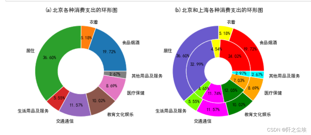

 所有地区支出对比

colors=['red','yellow','slateblue','lawngreen','magenta','green','orange','cyan','pink','gold']p1=plt.pie(df["北京"],labels=df["支出项目"],autopct="%1.2f%%",radius=2,pctdistance=0.95,           colors=colors,wedgeprops=dict(linewidth=1,width=0.3,edgecolor="w"))p2=plt.pie(df["上海"],autopct="%1.2f%%",radius=1.7,pctdistance=0.9,           colors=colors,wedgeprops=dict(linewidth=1,width=0.3,edgecolor="w"))p3=plt.pie(df["天津"],autopct="%1.2f%%",radius=1.4,pctdistance=0.9,           colors=colors,wedgeprops=dict(linewidth=1,width=0.3,edgecolor="w"))p4=plt.pie(df["重庆"],autopct="%1.2f%%",radius=1.1,pctdistance=0.85,           colors=colors,wedgeprops=dict(linewidth=1,width=0.3,edgecolor="w"))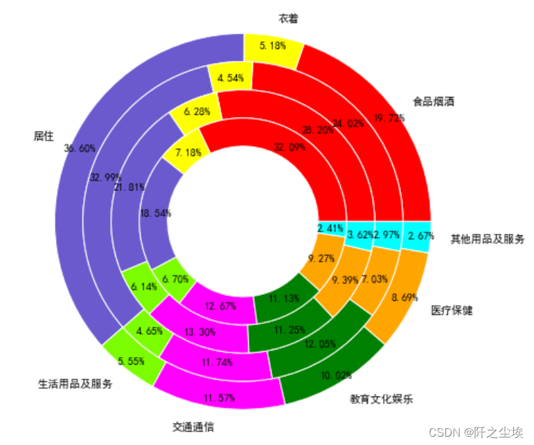

数值型数据的可视化

前面刚刚都是分类的数据进行可视化，现在是数值型数据的可视化，常见的图有直方图，核密度图，箱线图，小提琴图，点图等。

先导入包，读取案例数据

#导入相关模块import numpy as npimport pandas as pdimport matplotlib.pyplot as pltimport seaborn as sns#显示中文plt.rcParams ['font.sans-serif'] ='SimHei'plt.rcParams ['axes.unicode_minus']=False               #显示负号sns.set_style("darkgrid",{ "font.sans-serif":['KaiTi', 'Arial']})  #设置画图风格（奶奶灰）

df=pd.read_csv('example2_3.csv',encoding='gbk')df.head()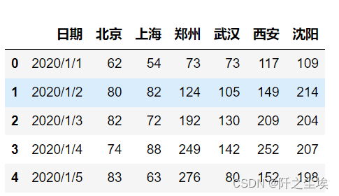

直方图和核密度图

直方图，每个地区用不同的样式

#直方图plt.subplots(2,3,figsize=(12,8))plt.subplot(231)sns.histplot(df['北京'])plt.title("(a)默认绘制（y轴是频数）")plt.subplot(232)sns.histplot(df['上海'],kde=True,stat='frequency')  #显示核密度曲线，y轴为频率plt.title("(b)显示核密度（y轴是频率）")plt.subplot(233)sns.histplot(df['郑州'],bins=20,kde=True,stat='density')  #分成20个箱子，y为密度（面积为1）plt.title("(c)分成20组（y轴为密度）")plt.subplot(234)sns.histplot(df['武汉'],bins=30,kde=True,stat='probability') #y为概率（总和为1）plt.title("(d)分成30组（y轴为概率）")plt.subplot(235)sns.histplot(df['西安'],bins=30,kde=True,stat='density',element='poly')  #直方图尖峰plt.title("(e)直方图尖峰")plt.subplot(236)sns.histplot(df['沈阳'],bins=30,kde=True,stat='density',element='step') #直方图阶梯plt.title("(f)直方图梯形")plt.tight_layout()plt.show()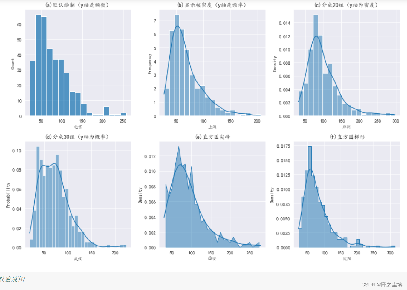

 核密度图

核密度曲线其实大概就是直方图的平滑出的一条线，可以看数据的分布形状。平滑程度取决于带宽bw，bw越大越平滑。

#核密度图plt.subplots(1,3,figsize=(15,4))plt.subplot(131)sns.kdeplot(df['北京'],bw_adjust=0.2)plt.title('(a)bw=0.2')plt.subplot(132)sns.kdeplot(df['北京'],bw_adjust=0.5)plt.title('(b)bw=0.5')plt.subplot(133)sns.kdeplot('北京',data=df,bw_method=0.5)plt.title('(c)bw=0.5')plt.show()

 可以把核密度图画到一个图上对比，

先把数据融合，也就是将不同列变成一个特征变量

#融合数据df2=pd.melt(df,value_vars=['北京','上海','郑州','武汉','西安','沈阳'],var_name='城市',value_name='AQI')df2

#核密度曲线比较plt.subplots(2,1,figsize=(8,6))plt.subplot(211)sns.kdeplot('AQI',hue='城市',lw=0.6,data=df2)plt.title('(a)曲线无填充')plt.subplot(212)sns.kdeplot('AQI',hue='城市',shade=True,alpha=0.1,lw=0.6,data=df2)plt.title('(b)曲线下填充阴影')plt.tight_layout()plt.show()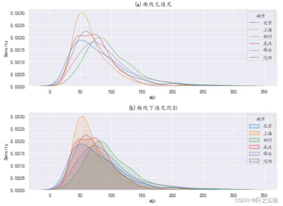

箱线图

plt.figure(figsize=(8,5))sns.boxplot(x='城市',y='AQI',width=0.6,saturation=0.9,    #颜色饱和度            fliersize=2,linewidth=0.8,notch=False,palette='Set2',orient='v',data=df2)plt.xticks(fontsize=15,rotation=10)plt.show()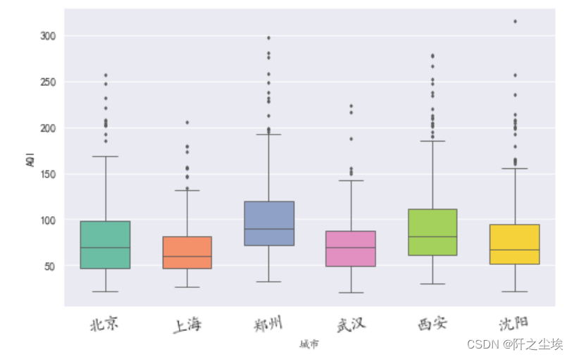

 小提琴图

小提琴图比箱线图好的位置在于可以看核密度估计

##小提琴图plt.figure(figsize=(8,5))sns.violinplot(x='城市',y='AQI',width=0.8,saturation=0.9,    #饱和度            fliersize=2,linewidth=0.8,palette='Set2',orient='v',inner='box',data=df2)plt.xticks(fontsize=15,rotation=10)plt.show()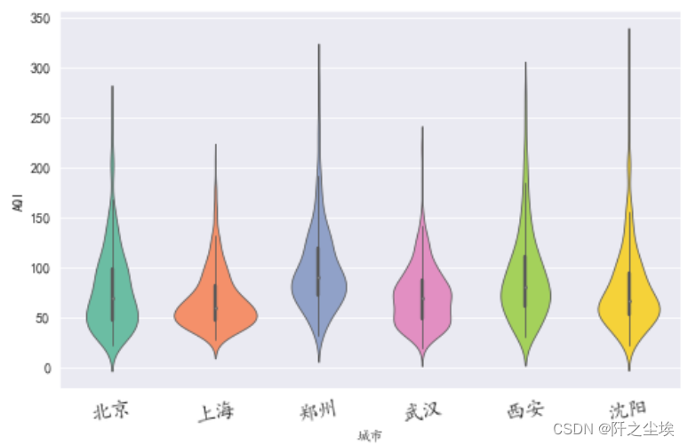

点图

点图可以很方便的看离群点

####点图plt.subplots(1,2,figsize=(10,5))plt.subplot(121)sns.stripplot(x='城市',y='AQI',jitter=False,size=2,data=df2)plt.title("(a)原始数据点图")plt.subplot(122)sns.stripplot(x='城市',y='AQI',size=2,data=df2)plt.title("(b)原始扰动后点图")plt.show()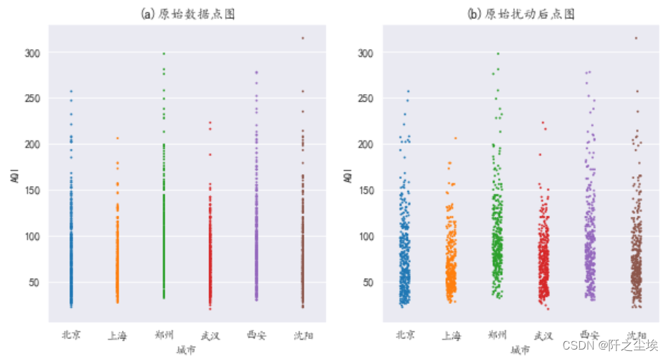

 变量间关系可视化

前面都是单个变量或者是多个分类变量的可视化，若是数值型变量之间的关系可视化应该用如下图形。

读取案例数据

df=pd.read_csv('example2_4.csv',encoding='gbk')df.head()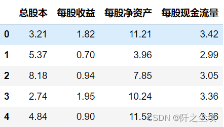

散点图

#散点图plt.subplots(1,2,figsize=(10,4))plt.subplot(121)sns.regplot(x=df['总股本'],y=df["每股收益"],fit_reg=False,marker='.',data=df)plt.title('(a)普通散点图')plt.subplot(122)sns.regplot(x=df['总股本'],y=df["每股收益"],fit_reg=True,marker='.',data=df)      #添加回归线plt.title('(b)加上回归线和置信区间')plt.show()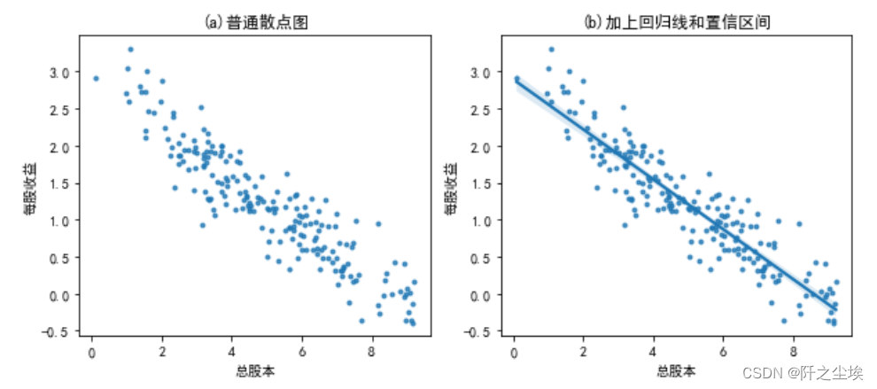

 封箱的散点图

#六边形封箱的散点图sns.jointplot(x=df['总股本'],y=df["每股收益"],kind='hex',height=5,ratio=3,data=df)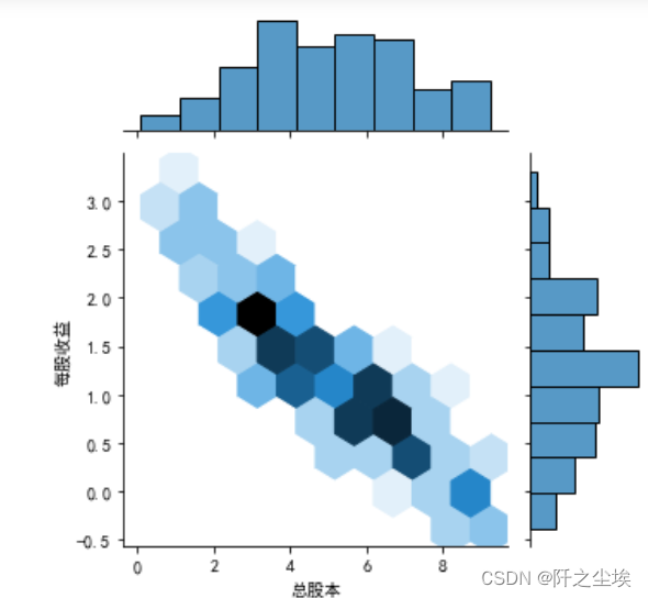

 散点图矩阵

sns.pairplot(df[["总股本",'每股收益','每股净资产','每股现金流量']],height=2,diag_kind='kde',markers='.',kind='reg')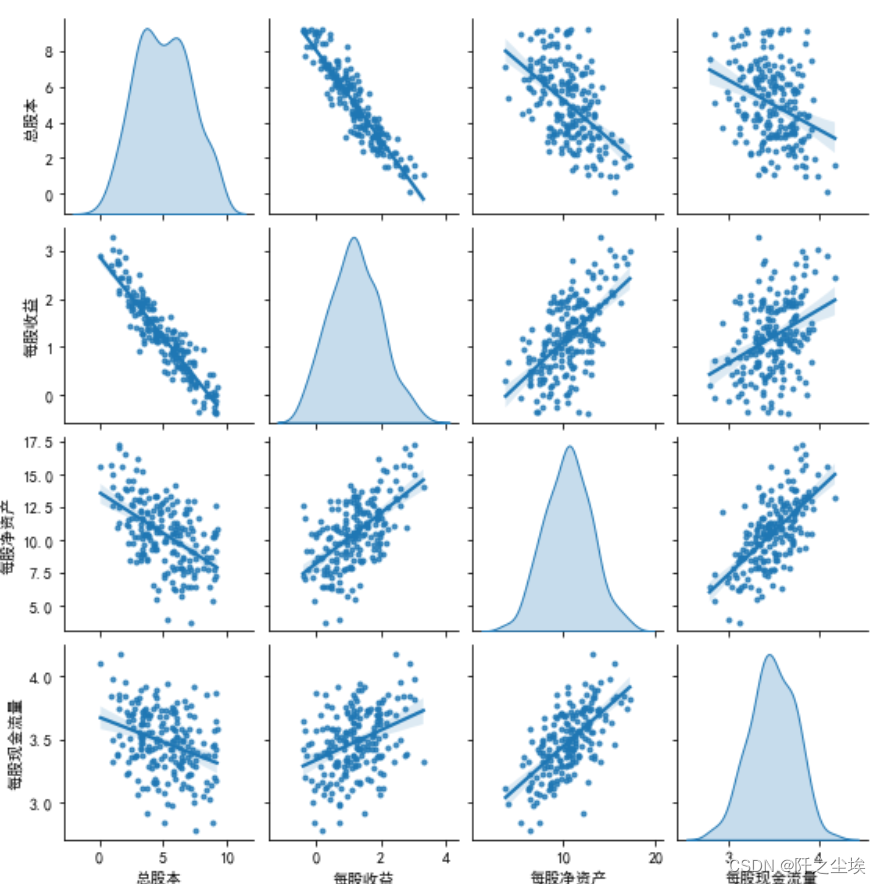

 气泡图

气泡图可以描述三个变量之间的关系

#气泡图plt.figure(figsize=(8,5))plt.scatter(x='每股收益',y='每股净资产',c='总股本',s=df["总股本"]*60,             cmap="Blues",edgecolors='k',lw=0.5,alpha=0.6,data=df)plt.colorbar()plt.xlabel('每股收益',fontsize=12)plt.ylabel('每股净资产',fontsize=12)plt.title("总股本——气泡图",fontsize=14)plt.show()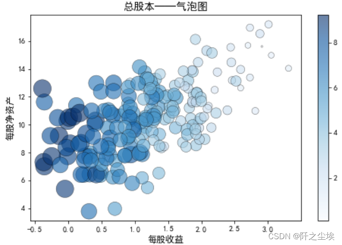

 3D散点图

#3D散点图ax3d=plt.figure(figsize=(10,7)).add_subplot(111,projection="3d")ax3d.scatter(df['每股收益'],df['每股净资产'],df['总股本'],color='black',marker="*",s=50)ax3d.set_xlabel('每股收益',fontsize=12)ax3d.set_ylabel('每股净资产',fontsize=12)ax3d.set_zlabel('总股本',fontsize=12)plt.xlabel('x=每股收益',fontsize=12)plt.ylabel('y=每股净资产',fontsize=12)#plt.zlabel('z=总股本',fontsize=12)plt.show()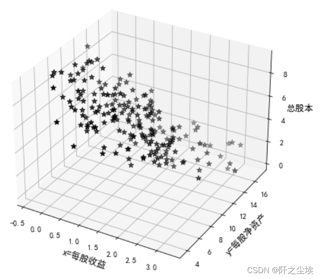

样本相似性可视化

读取案例数据

df=pd.read_csv('example2_2.csv',encoding='gbk')df.head(10)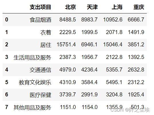

 折线图

dfs=[df['北京'],df["天津"],df['上海'],df['重庆']]sns.lineplot(data=dfs,marker=True)plt.xlabel('支出项目')plt.ylabel('支出金额')plt.xticks(range(8),df['支出项目'])plt.show()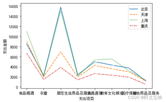

雷达图

 还可以用雷达图看

attributes=list(df.columns[1:])values=list(df.values[:,1:])names=list(df.values[:,0])angles=[n / float(len(names))*2*np.pi for  n in range(len(names))]angles+=angles[:1]values=np.asarray(values)values=np.concatenate([values.T,values.T[:,0:1]],axis=1)

sns.set_style("darkgrid",{ "font.sans-serif":['KaiTi', 'Arial']})plt.figure(figsize=(8,8),dpi=100)for i in range(4):    ax=plt.subplot(2,2,i+1,polar=True)    ax.plot(angles,values[i])        ax.set_yticks(np.arange(500,16000,3500))    ax.set_xticks(angles[:-1])    ax.set_xticklabels(names)    ax.set_title(attributes[i],fontsize=12,color='red')    plt.tight_layout()plt.show()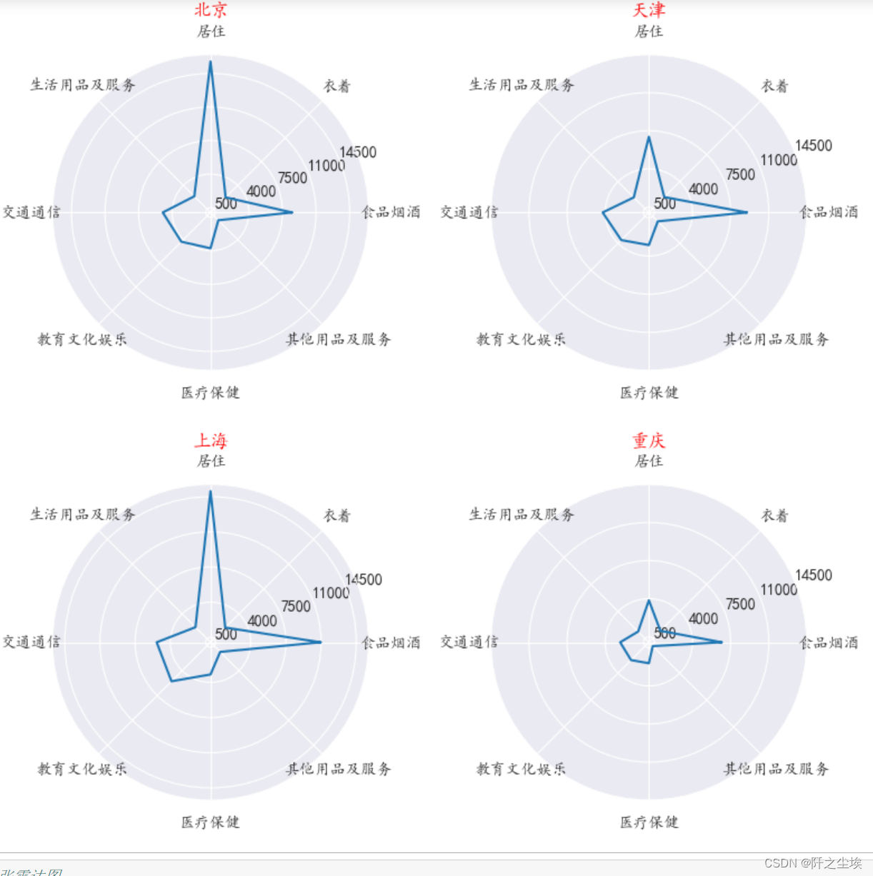

 画在一张雷达图上，分布对比

#一张雷达图labels=np.array(df['支出项目'])datalenth=8df1=np.array(df['北京'])df2=np.array(df['天津'])df3=np.array(df['上海'])df4=np.array(df['重庆'])angles=np.linspace(0,2*np.pi,datalenth,endpoint=False)df1=np.concatenate((df1,[df1[0]]))df2=np.concatenate((df2,[df2[0]]))df3=np.concatenate((df3,[df3[0]]))df4=np.concatenate((df4,[df4[0]]))angles=np.concatenate((angles,[angles[0]]))

plt.figure(figsize=(6,6),facecolor='lightyellow',dpi=100)plt.polar(angles,df1,"r--",lw=1,label="北京")plt.polar(angles,df2,"b",lw=1,label="天津")plt.polar(angles,df3,"k",lw=1,label="上海")plt.polar(angles,df4,"g",lw=1,label="重庆")plt.thetagrids(range(0,360,45),labels)plt.grid(linestyle="-",lw=0.5,color="gray",alpha=0.5)  #网格plt.legend(loc="upper right",bbox_to_anchor=(1.1,1.1))   #图例plt.show()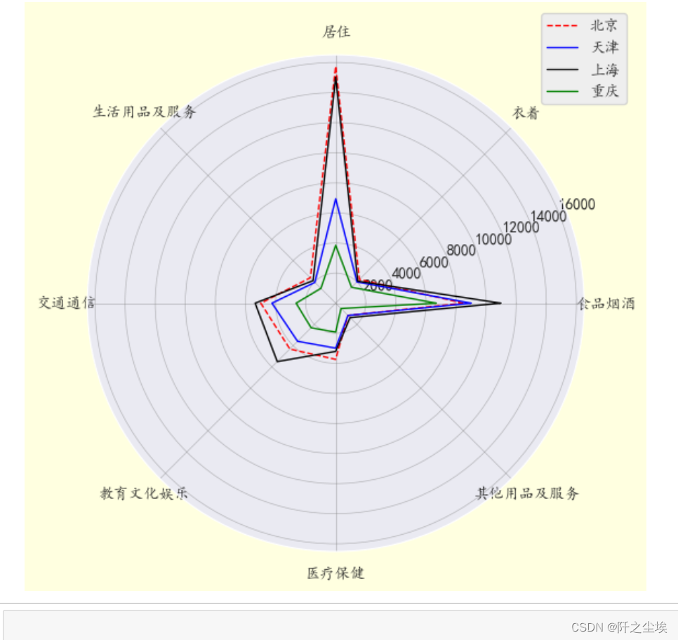

时间序列可视化

时间序列数据的特点就是连续，要采用折线图表示发展趋势。

df=pd.read_csv('example2_6.csv',encoding='gbk')df['年份']=pd.to_datetime(df["年份"],format="%Y")df=df.set_index('年份')df.head()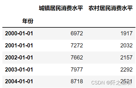

折线图

plt.figure(figsize=(10,4))plt.plot(df['城镇居民消费水平'],marker='o')plt.plot(df['农村居民消费水平'],marker='+')plt.legend(df.columns,loc='upper left',fontsize=10)plt.title('消费水平变化',fontsize=16)plt.xlabel('日期',fontsize=12)plt.ylabel('消费指标',fontsize=12)plt.show()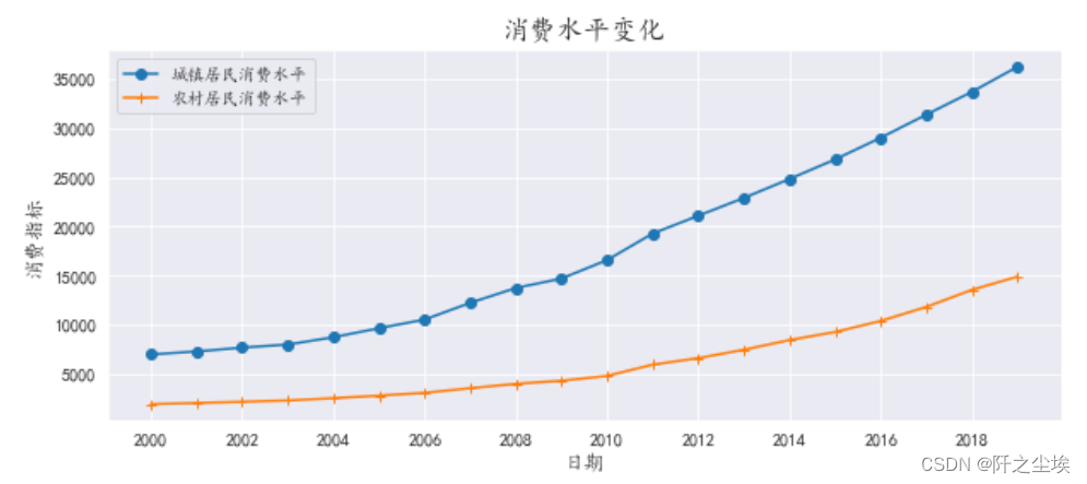

面积图

plt.figure(figsize=(10,4))plt.stackplot(df.index,df['城镇居民消费水平'],df['农村居民消费水平'],labels=df.columns)   #堆积面积图,数值大的在下面plt.legend(df.columns,loc='upper left',fontsize=10)plt.title('消费水平变化',fontsize=16)plt.xlabel('日期',fontsize=12)plt.ylabel('消费指标',fontsize=12)plt.show()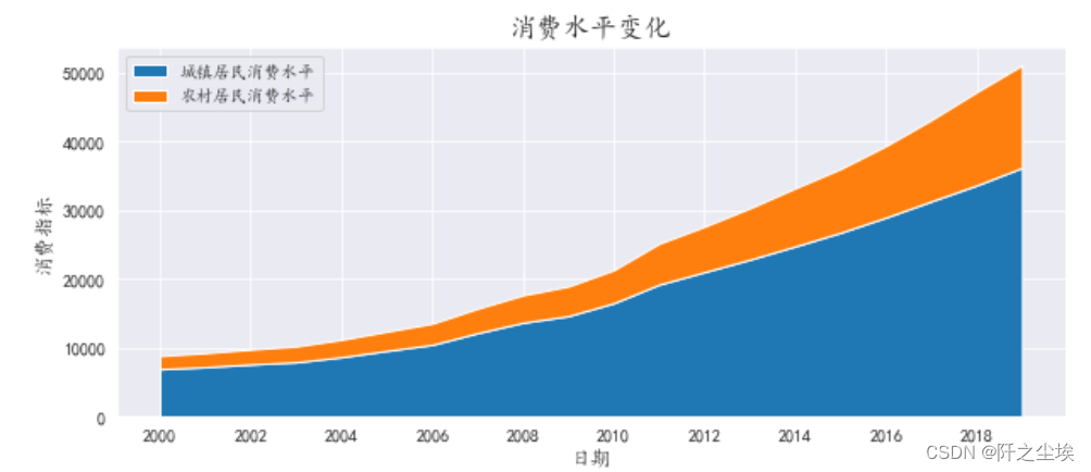

多子图

画子图的方法有很多，学一种均匀分布的和不对称分布的就行。

均匀分布的多子图，每个图都一样大

np.random.seed(1010)plt.subplots(nrows=2,ncols=2,figsize=(10,7))plt.subplot(221)plt.scatter(x=range(100),y=np.random.randint(low=0,high=100,size=100),marker="^",c='r')plt.subplot(222)plt.hist(np.random.normal(loc=5,scale=10,size=100),bins=10,color='lightgreen')plt.subplot(223)plt.plot(range(20),np.random.normal(5,10,20),marker="o",linestyle="-.",linewidth=2,markersize=5)plt.subplot(224)plt.bar(x=range(5),height=range(5,0,-1),color=['cyan','pink'])plt.show()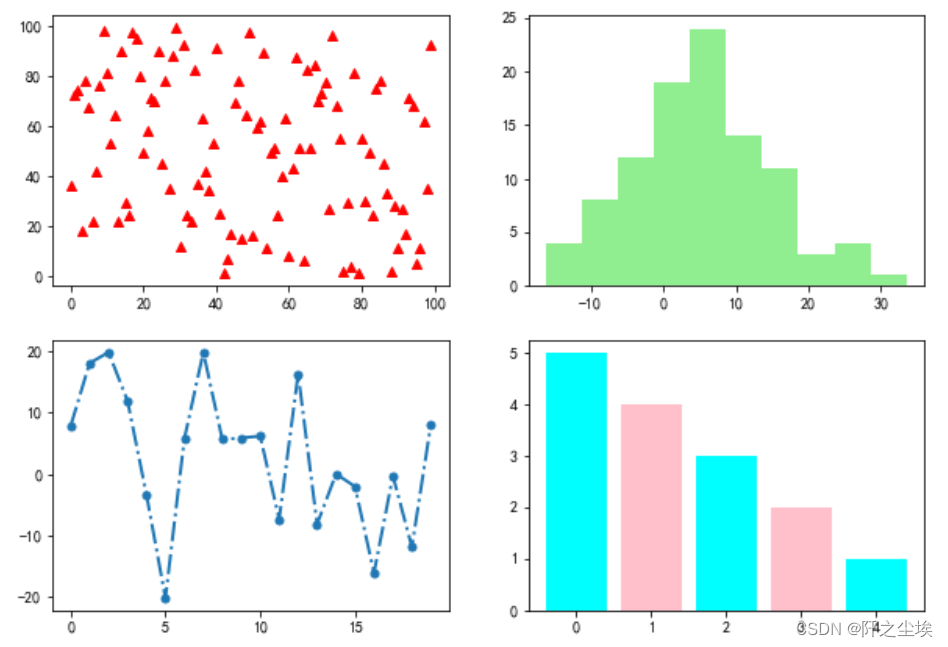

还可以把有的小图位置占多个图 ，这样就实现了不均匀的子图，大小不一

fig=plt.figure(figsize=(6,5))grid=plt.GridSpec(3,3)plt.subplot(grid[0,:2])plt.scatter(x=range(100),y=np.random.randint(low=0,high=100,size=100),marker="^",c='r')plt.subplot(grid[0,2])plt.subplot(grid[1,:1])plt.subplot(grid[1,1:])plt.plot(range(20),np.random.normal(5,10,20),marker="o",linestyle="-.",linewidth=2,markersize=5)plt.subplot(grid[2,:3])plt.tight_layout()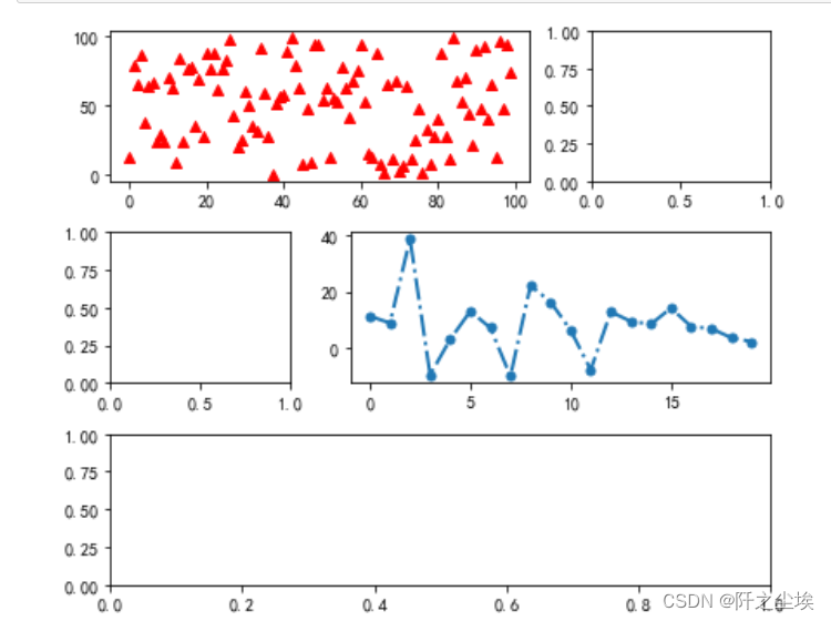

 其他参数

plt画图有很多元素，这些参数需要了解一下，比如坐标轴，标题，xy轴标签等等

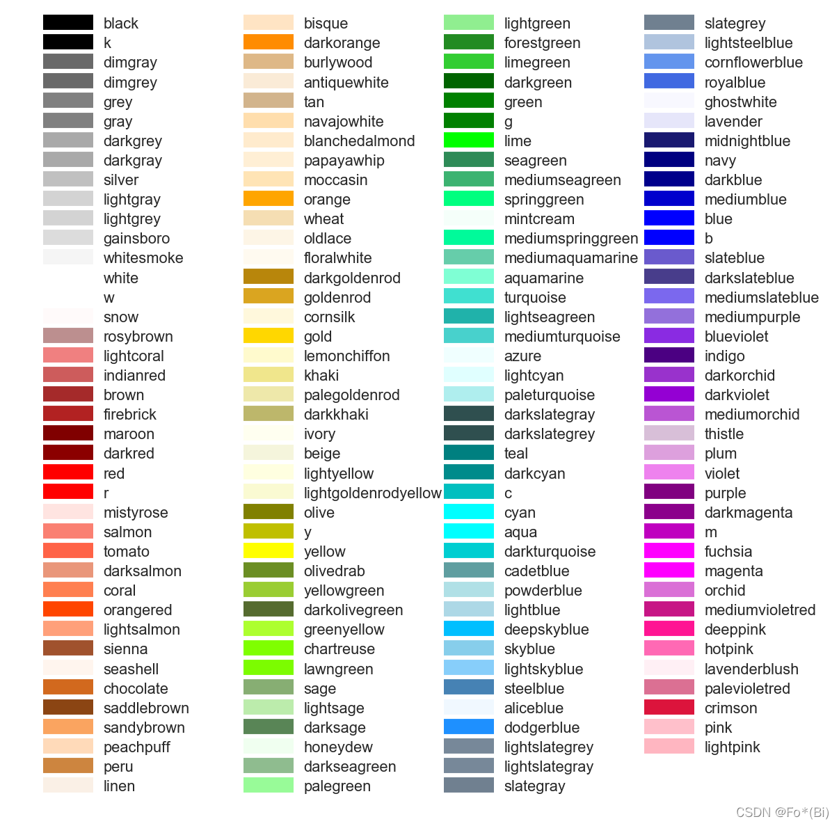
还有点的形状，线的样式，颜色等等参数。

color 颜色
linestyle 线条样式
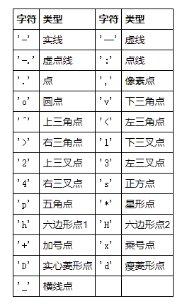
marker 标记风格
markerfacecolor 标记颜色
markersize 标记大小 等等

#坐标轴plt.xlim(-1,7)#x轴范围plt.ylim(-1.5,1.5)#y轴范围plt.axis([-2,8, -2,2])#xy范围plt.axis('tight')#图像紧一点,equal扁一点plt.xscale('log')#x轴对数plt.xticks(np.arrange(0,12,step=1))#x轴的刻度plt.xticks(rotation=40)    #x轴旋转度plt.tick_params(axis='both',labelsize=15)#刻度样式plt.title('A big title',fontsize=20)#设置大标题plt.xlabel('x',fontsize=15)#x轴标签plt.ylabel('sin(x)',fontsize=15)#y标签plt.plot(x,np.sin(x),'b-',label='sin')#设置线名称plt.plot(x,np.cos(x),'r--',label='cos')plt.legend(loc='best',frameon=True,fontsize=15)#图像最好的位置,网格显示plt.text(3.5,0.5,'y=sinx',fontsize=15)#添加文字plt.annotate('local min',xy=(1.5*np.pi,-1),xytext=(4.5,0),           #加箭头    arrowprops=dict(facecolor='black',shrink=0.1),)

点形状

线条样式

颜色